Exercise 2 - Using edgeR in R
Introduction
Here we will explore some of the potential of edgeR to perform differential expression analysis in more complex settings. We will be using data from Fu et al., 2015. You can obtain the raw data, and some processed data like gene counts from here. For your convenience, these have already been provided
In this study the authors studied evolution of gene expression during lactogenesis. The data is a set of RNA-seq samples of two different tissues (basal and luminal) in the mammary gland, at three different time points (virgin, pregnant and lactating).
Load the count data
We start by importing the counts table into R. It contains the gene identifier (in this case it is not an Ensembl identifier, but Entrez gene ID), the gene length, and then the counts for each sample.
rawdata <- read.delim("edgeR_example4_GSE60450_Lactation-GenewiseCounts.tab", sep = "\t")
head(rawdata)
##   EntrezGeneID Length  DG  DH  DI  DJ  DK  DL  LA  LB  LC  LD  LE  LF
## 1       497097   3634 438 300  65 237 354 287   0   0   0   0   0   0
## 2    100503874   3259   1   0   1   1   0   4   0   0   0   0   0   0
## 3    100038431   1634   0   0   0   0   0   0   0   0   0   0   0   0
## 4        19888   9747   1   1   0   0   0   0  10   3  10   2   0   0
## 5        20671   3130 106 182  82 105  43  82  16  25  18   8   3  10
## 6        27395   4203 309 234 337 300 290 270 560 464 489 328 307 342
dim(rawdata)
## [1] 27179 14
One of the first things you should do with your data is to have a global overview of it, as unbiased as possible from your final goals. For example, you may want to detect potentially problematic samples, or possible confounding elements.
library(edgeR)
## Loading required package: limma
#We create an edgeR object, with the counts and information on the genes (ID and length)
y <- DGEList(counts=rawdata[,3:14], genes=rawdata[,1:2])
#We now perform normalization steps, which is totally independent from our experimental design
y <- calcNormFactors(y)
#Now we can see the scaling factors: these should be "reasonably" similar among all samples
y$samples
##    group lib.size norm.factors
## DG     1 23227641    1.2387271
## DH     1 21777891    1.2179397
## DI     1 24100765    1.1279619
## DJ     1 22665371    1.0788322
## DK     1 21529331    1.0377926
## DL     1 20015386    1.0772749
## LA     1 20392113    1.3530159
## LB     1 21708152    1.3577394
## LC     1 22241607    1.0024180
## LD     1 21988240    0.9210201
## LE     1 24723827    0.5344186
## LF     1 24657293    0.5375196
# It is common to remove low expressed genes
# In this case we remove genes that do NOT have
# at least 1 CPM in at least 2 samples
# isexpr <- rowSums(cpm(y)>1) >= 2
# y <- y[isexpr, , keep.lib.sizes=FALSE]
# This reduces the number of necessary tests

#you can get normalized counts like this:
normcounts<-cpm(y, normalized.lib.sizes = T)
#You can also get it in log scale like this:
#normcounts<-cpm(y, normalized.lib.sizes = T, log = T)

#We can see a PcoA (MDS plot) to see how the samples relate to each other
plotMDS(y)
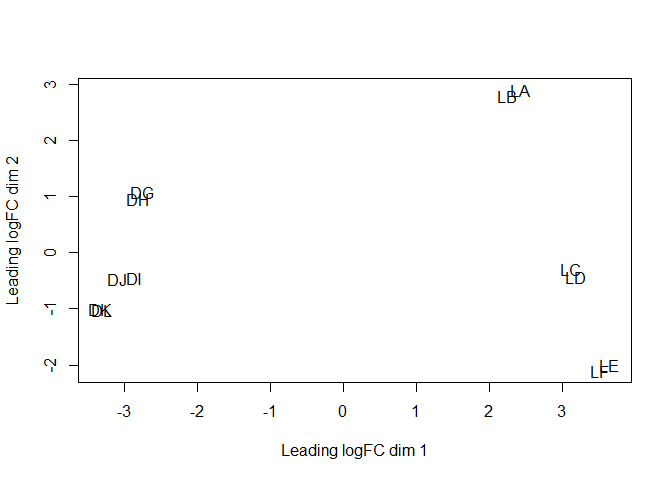
Question: What does this global overview tell you?
Click Here to see the answer
The scaling factors are a bit different between samples, but still seem "reasonably" similar. The MDS plot seems to indicate two major axis of separation, where samples are grouped two by two.Note: The PCoA (MDS) plot is not the same as PCA plot, and it is considered to be a more robust way to display distances between samples.
But we still don’t know the meaning of each sample, so we need to also load metadata associated to the samples.
metadata <- read.delim("edgeR_example4_GSE60450_Lactation_metadata.tab", header=TRUE)
metadata
##    Sample CellType   Status Lane
## 1      DG        B   virgin    2
## 2      DH        B   virgin    2
## 3      DI        B pregnant    2
## 4      DJ        B pregnant    2
## 5      DK        B  lactate    2
## 6      DL        B  lactate    2
## 7      LA        L   virgin    1
## 8      LB        L   virgin    1
## 9      LC        L pregnant    1
## 10     LD        L pregnant    1
## 11     LE        L  lactate    1
## 12     LF        L  lactate    1
Question: Do you see a potential issue in the metadata, regarding the experimental design?
Click Here to see the answer
The cell type is deeply correlated with the sequencing lane. Therefore, we cannot distinguish the technical variation caused by the sequencing lane from the true biological variation. It is well accepted that sequencing lanes have low and well identified technical variation, but it is nonetheless a potential confounder in the experiment.Question: How do you interpret the MDS, considering the metadata information?
Click Here to see the answer
The major axis of separation is the cell type, and the second axis is the developmental stage, with a "logical" transition between virgin, pregnant and lactating. Also, this second axis seems to be more relevant in luminal cells. The replicates seem to group together, as expected.Let’s first start simple, and make a pairwise comparison between the two cell types, using GLM (note that we could also use a classical non-GLM method). In this case, we have 6 replicates for each cell type.
Generalized Linear Models (GLM) are an extension of traditional linear models to allow for non-normal distributions (such as poisson or negative binomial). To use the GLM we need to define the variables to be considered in the model, which we call a design.
design <- model.matrix(~ CellType, data=metadata)
rownames(design) <- colnames(y)
design
##    (Intercept) CellTypeL
## DG           1         0
## DH           1         0
## DI           1         0
## DJ           1         0
## DK           1         0
## DL           1         0
## LA           1         1
## LB           1         1
## LC           1         1
## LD           1         1
## LE           1         1
## LF           1         1
## attr(,"assign")
## [1] 0 1
## attr(,"contrasts")
## attr(,"contrasts")$CellType
## [1] "contr.treatment"
#Alternatively, you can also define:
#CellType <- factor(c("B","B","B","B","B","B","L","L","L","L","L","L"))
#design <- model.matrix(~ CellType)
#rownames(design) <- colnames(y)
Here, we have a single variable with two values. Our GLM model will therefore be composed of a binary variable, which is 1 when the cell type is “L” and 0 when the cell type is “B”.
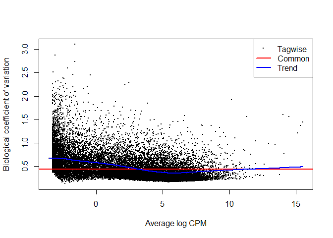
The next step in edgeR is to estimate the dispersion of the gene expression. As we discussed before, it makes use of some assumptions, such as that most genes should not be differentially expressed, and dispersion should not be dependent on the relative expression of the gene.
y <- estimateDisp(y, design, robust=TRUE)
#Type ?estimateDisp() to see more information

#This shows the curve fitting to reestimate the dispersion
plotBCV(y)
Next, edgeR fits the GLM model for each gene (like we fit linear models using regression and least squeares, but with more sophisticated iterative methods).
The differential expression test consists basically in identifying if a specific chosen variable (or combinations of variables) have a significant role in the fitting of the GLM. For this, it also takes in consideration the dispersion estimates calculated before.
By default, the variable that is checked for significance is the last in the design matrix. In this case, there is only one. We’re testing if being a specific CellType has any bearing in gene expression. For the genes where that’s the case, the gene expression in the samples of one cell type must be significantly different than in the samples for the other cell type (which is what we want).
#The recommended fitting procedure in edgeR returns
# Quasi-F as statistic for significance in the GLM
fit <- glmQLFit(y, design, robust=TRUE)
qlt <- glmQLFTest(fit)

# The topTags function gives the genes where the variable was significant
# if we want all genes, we need to ask for it using the n parameter
# dim(rawdata)[[1]] contains the total number of genes (number of lines)
topgenes<-topTags(qlt, n=dim(rawdata)[[1]])

#How many are significant between the cell lines?
table(topgenes$table$FDR<0.05)
##
## FALSE  TRUE
## 17517  9662
Question: For how many different genes did the GLM model consider the variable CellType significant (the differentially expressed genes we’re looking for)?
Click Here to see the answer
A whopping 9662 genes! Depending on what we want, we may be stricter with choosing an FDR. Also, we can choose based on the estimated LogFC.Next, let’s add the developmental stage (status) as a confounding variable in the design.
#It's best to start from scratch
y <- DGEList(counts=rawdata[,3:14], genes=rawdata[,1:2])
y <- calcNormFactors(y)

#The last Variable is always the one of interest
#Confounding variables can be added before, separated by '+'
design <- model.matrix(~ Status + CellType, data=metadata)
rownames(design) <- colnames(y)
design
##    (Intercept) Statuspregnant Statusvirgin CellTypeL
## DG           1              0            1         0
## DH           1              0            1         0
## DI           1              1            0         0
## DJ           1              1            0         0
## DK           1              0            0         0
## DL           1              0            0         0
## LA           1              0            1         1
## LB           1              0            1         1
## LC           1              1            0         1
## LD           1              1            0         1
## LE           1              0            0         1
## LF           1              0            0         1
## attr(,"assign")
## [1] 0 1 1 2
## attr(,"contrasts")
## attr(,"contrasts")$Status
## [1] "contr.treatment"
##
## attr(,"contrasts")$CellType
## [1] "contr.treatment"
In this case, when estimating the dispersion and fitting the GLM, it will also consider the status.
y <- estimateDisp(y, design, robust=TRUE)
fit <- glmQLFit(y, design, robust=TRUE)
qlt <- glmQLFTest(fit)
topgenes<-topTags(qlt, n=dim(rawdata)[[1]])

#How many are significant between the cell lines?
table(topgenes$table$FDR<0.05)
##
## FALSE  TRUE
## 15885 11294
Question: How many genes do you get now?
Click Here to see the answer
Even more genes: 11294!What about the status of the mouse? In this case, we have three values (virgin, pregnant, lactating).
Task: Make a design matrix to test status, controlling for cell type.
Click Here to see the answer
design <- model.matrix(~ CellType + Status, data=metadata)
rownames(design) <- colnames(y)
design
##    (Intercept) CellTypeL Statuspregnant Statusvirgin
## DG           1         0              0            1
## DH           1         0              0            1
## DI           1         0              1            0
## DJ           1         0              1            0
## DK           1         0              0            0
## DL           1         0              0            0
## LA           1         1              0            1
## LB           1         1              0            1
## LC           1         1              1            0
## LD           1         1              1            0
## LE           1         1              0            0
## LF           1         1              0            0
## attr(,"assign")
## [1] 0 1 2 2
## attr(,"contrasts")
## attr(,"contrasts")$CellType
## [1] "contr.treatment"
##
## attr(,"contrasts")$Status
## [1] "contr.treatment"
Question: If you do a test with this design, what will you be testing?
Click Here to see the answer
By default, the test checks for the last element in the design matrix, which is Statusvirgin. In this case, it will check whether being a virgin (or not) significantly changes baseline gene expression (in this case, controlling for the cell type).You can do combined tests. For example, if you want to see genes significant for Statuspregnant or Statusvirgin (any of the two), you can select the last 2 columns (you just need to do that in the testing phase, as the model fitting is already done):
qlt <- glmQLFTest(fit, coef=c(3,4))
topgenes<-topTags(qlt, n=dim(rawdata)[[1]])
table(topgenes$table$FDR<0.05)
##
## FALSE  TRUE
## 14869 12310
Note: In the previous test, since lactating is mutually exclusive from pregnant and virgin (therefore, dependent), the last test is equivalent to ask for any gene differentially expressed between any of the status, controlling for cell type.
The problem with this setting is that it starts getting complicated to do certain tests. For example, how do you test for genes differentially expressed between virgin and pregnant? Moreover, interpreting the meaning of the baseline gets complex, as it is a mixture of several factors.
Note: You can always make a differential analysis test using just the samples you want to compare. Adding more samples and variables into the same model allow you to control for these variables, which you would otherwise ignore.
Making the combinations explicit in the model make it probably easier to interpret.
metadata$cell_status<-paste(metadata$CellType, metadata$Status, sep = ".")
metadata
##    Sample CellType   Status Lane cell_status
## 1      DG        B   virgin    2    B.virgin
## 2      DH        B   virgin    2    B.virgin
## 3      DI        B pregnant    2  B.pregnant
## 4      DJ        B pregnant    2  B.pregnant
## 5      DK        B  lactate    2   B.lactate
## 6      DL        B  lactate    2   B.lactate
## 7      LA        L   virgin    1    L.virgin
## 8      LB        L   virgin    1    L.virgin
## 9      LC        L pregnant    1  L.pregnant
## 10     LD        L pregnant    1  L.pregnant
## 11     LE        L  lactate    1   L.lactate
## 12     LF        L  lactate    1   L.lactate
Finally, to overcome the issue of the baseline, we can force the model to have a zero baseline.
design <- model.matrix(~ 0 + cell_status, data=metadata)
rownames(design) <- colnames(y)
design
##    cell_statusB.lactate cell_statusB.pregnant cell_statusB.virgin
## DG                    0                     0                   1
## DH                    0                     0                   1
## DI                    0                     1                   0
## DJ                    0                     1                   0
## DK                    1                     0                   0
## DL                    1                     0                   0
## LA                    0                     0                   0
## LB                    0                     0                   0
## LC                    0                     0                   0
## LD                    0                     0                   0
## LE                    0                     0                   0
## LF                    0                     0                   0
##    cell_statusL.lactate cell_statusL.pregnant cell_statusL.virgin
## DG                    0                     0                   0
## DH                    0                     0                   0
## DI                    0                     0                   0
## DJ                    0                     0                   0
## DK                    0                     0                   0
## DL                    0                     0                   0
## LA                    0                     0                   1
## LB                    0                     0                   1
## LC                    0                     1                   0
## LD                    0                     1                   0
## LE                    1                     0                   0
## LF                    1                     0                   0
## attr(,"assign")
## [1] 1 1 1 1 1 1
## attr(,"contrasts")
## attr(,"contrasts")$cell_status
## [1] "contr.treatment"
Now, we need to be carefull when choosing the variables to check for significance, because simply choosing the column indicates whether that variable is different from zero (which is true for all expressed genes!).
Question: How many genes you get with the default test for glmQLFtest?
Click Here to see the answer
y <- DGEList(counts=rawdata[,3:14], genes=rawdata[,1:2])
y <- calcNormFactors(y)
y <- estimateDisp(y, design, robust=TRUE)
fit <- glmQLFit(y, design, robust=TRUE)
qlt <- glmQLFTest(fit)
topgenes<-topTags(qlt, n=dim(rawdata)[[1]])
table(topgenes$table$FDR<0.05)
##
## FALSE  TRUE
##  5788 21391
Now we need to create new variables to test if they are different from zero. For example, to see genes differentially expressed between virgin and pregnant in Luminal cells:
y <- DGEList(counts=rawdata[,3:14], genes=rawdata[,1:2])
y <- calcNormFactors(y)
y <- estimateDisp(y, design, robust=TRUE)
fit <- glmQLFit(y, design, robust=TRUE)
qlt <- glmQLFTest(fit, contrast=makeContrasts(cell_statusL.virgin - cell_statusL.pregnant, levels=design))
topgenes<-topTags(qlt, n=dim(rawdata)[[1]])
table(topgenes$table$FDR<0.05)
##
## FALSE  TRUE
## 20374  6805
Like before, you can choose different variables to test simultaneously. For example, you may want to perform ANOVA-like tests, to see for genes that vary among any combination of values of a variable.
#ANOVA-Like for L samples (it tests if any of these combinations has logFC != 0)
con <- makeContrasts(cell_statusL.pregnant - cell_statusL.lactate,
                     cell_statusL.virgin - cell_statusL.lactate,
                     cell_statusL.virgin - cell_statusL.pregnant, levels=design)
anov <- glmQLFTest(fit, contrast=con)
topgenes<-topTags(anov, n=dim(rawdata)[[1]])
table(topgenes$table$FDR<0.05)
##
## FALSE  TRUE
## 16156 11023
As a final example, we will see that using GLM models, you can also check for interaction between variables.
y <- DGEList(counts=rawdata[,3:14], genes=rawdata[,1:2])
y <- calcNormFactors(y)
#This design includes interaction of Cell Type and Status
design <- model.matrix(~ CellType*Status, data=metadata)
design
##    (Intercept) CellTypeL Statuspregnant Statusvirgin
## 1            1         0              0            1
## 2            1         0              0            1
## 3            1         0              1            0
## 4            1         0              1            0
## 5            1         0              0            0
## 6            1         0              0            0
## 7            1         1              0            1
## 8            1         1              0            1
## 9            1         1              1            0
## 10           1         1              1            0
## 11           1         1              0            0
## 12           1         1              0            0
##    CellTypeL:Statuspregnant CellTypeL:Statusvirgin
## 1                         0                      0
## 2                         0                      0
## 3                         0                      0
## 4                         0                      0
## 5                         0                      0
## 6                         0                      0
## 7                         0                      1
## 8                         0                      1
## 9                         1                      0
## 10                        1                      0
## 11                        0                      0
## 12                        0                      0
## attr(,"assign")
## [1] 0 1 2 2 3 3
## attr(,"contrasts")
## attr(,"contrasts")$CellType
## [1] "contr.treatment"
##
## attr(,"contrasts")$Status
## [1] "contr.treatment"
y <- estimateDisp(y, design, robust=TRUE)
fit <- glmQLFit(y, design, robust=TRUE)
#If you want to test for any type of interaction, then you can check for the last two columns
qlt <- glmQLFTest(fit, coef=c(5,6))
topgenes<-topTags(qlt, n=dim(rawdata)[[1]])
table(topgenes$table$FDR<0.05)
##
## FALSE  TRUE
## 18637  8542
Task: Using the code above as an example, try to replicate the paired Tumour/Normal analysis from Tuch et al, using edgeR. You can find the counts table in the complex folder.
Back
Back to previous page.