- Introduction
- 1. Background
- 2. Retrieving sequences
- 3. Sequence alignment
- 4. Distance-based analyses
- 5. Recombination
- 6. Maximum likelihood based analyses
- 7. Visualising trees
- 8. Time-stamped phylogenies
- 9. Bayesian reconstruction of time trees
- 10. Effective population size estimation
- 11. Structured populations
- 12. References
- Published with GitBook
Distances walkthrough
First load the libraries you need.
library(ape)
library(phangorn)
library(network)
## network: Classes for Relational Data
## Version 1.12.0 created on 2015-03-04.
## copyright (c) 2005, Carter T. Butts, University of California-Irvine
##                     Mark S. Handcock, University of California -- Los Angeles
##                     David R. Hunter, Penn State University
##                     Martina Morris, University of Washington
##                     Skye Bender-deMoll, University of Washington
##  For citation information, type citation("network").
##  Type help("network-package") to get started.
Load the multiple sequence alignment using read.dna from the ape library.
myalignment.filename <- "ray2000_pruned_degapped.fas"
myalignment <- read.dna(myalignment.filename,format="fasta",as.matrix=TRUE)
Calculate distances using the TN93 model.
myalignment.dist.tn93 <- dist.dna(myalignment,model="TN93",as.matrix=TRUE)
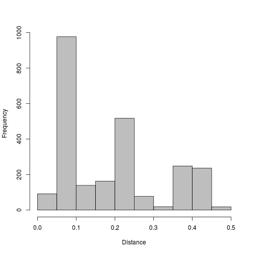
Plot out the distances.
hist(myalignment.dist.tn93[lower.tri(myalignment.dist.tn93)],xlab="Distance",ylab="Frequency",main="",col="grey")

Calculate a neighbour joining tree.
myalignment.tn93.nj <- nj(myalignment.dist.tn93)
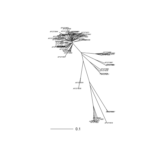
Plot the tree out and add a scale bar.
plot(myalignment.tn93.nj,"unrooted",cex=0.5)
add.scale.bar(length=0.1)

Bootstrap the alignment; we first define a function to make a tree from the alignment, then call boot.phylo.
maketree <- function(x) nj(dist.dna(x,model="TN93"))
myalignment.tn93.nj.boot <- boot.phylo(myalignment.tn93.nj,myalignment,maketree,B=100,block=3,trees=TRUE,quiet=FALSE,rooted=FALSE)
##
  |
  |                                                                 |   0%
  |
  |=                                                                |   1%
  |
  |=                                                                |   2%
  |
  |==                                                               |   3%
  |
  |===                                                              |   4%
  |
  |===                                                              |   5%
  |
  |====                                                             |   6%
  |
  |=====                                                            |   7%
  |
  |=====                                                            |   8%
  |
  |======                                                           |   9%
  |
  |======                                                           |  10%
  |
  |=======                                                          |  11%
  |
  |========                                                         |  12%
  |
  |========                                                         |  13%
  |
  |=========                                                        |  14%
  |
  |==========                                                       |  15%
  |
  |==========                                                       |  16%
  |
  |===========                                                      |  17%
  |
  |============                                                     |  18%
  |
  |============                                                     |  19%
  |
  |=============                                                    |  20%
  |
  |==============                                                   |  21%
  |
  |==============                                                   |  22%
  |
  |===============                                                  |  23%
  |
  |================                                                 |  24%
  |
  |================                                                 |  25%
  |
  |=================                                                |  26%
  |
  |==================                                               |  27%
  |
  |==================                                               |  28%
  |
  |===================                                              |  29%
  |
  |====================                                             |  30%
  |
  |====================                                             |  31%
  |
  |=====================                                            |  32%
  |
  |=====================                                            |  33%
  |
  |======================                                           |  34%
  |
  |=======================                                          |  35%
  |
  |=======================                                          |  36%
  |
  |========================                                         |  37%
  |
  |=========================                                        |  38%
  |
  |=========================                                        |  39%
  |
  |==========================                                       |  40%
  |
  |===========================                                      |  41%
  |
  |===========================                                      |  42%
  |
  |============================                                     |  43%
  |
  |=============================                                    |  44%
  |
  |=============================                                    |  45%
  |
  |==============================                                   |  46%
  |
  |===============================                                  |  47%
  |
  |===============================                                  |  48%
  |
  |================================                                 |  49%
  |
  |================================                                 |  50%
  |
  |=================================                                |  51%
  |
  |==================================                               |  52%
  |
  |==================================                               |  53%
  |
  |===================================                              |  54%
  |
  |====================================                             |  55%
  |
  |====================================                             |  56%
  |
  |=====================================                            |  57%
  |
  |======================================                           |  58%
  |
  |======================================                           |  59%
  |
  |=======================================                          |  60%
  |
  |========================================                         |  61%
  |
  |========================================                         |  62%
  |
  |=========================================                        |  63%
  |
  |==========================================                       |  64%
  |
  |==========================================                       |  65%
  |
  |===========================================                      |  66%
  |
  |============================================                     |  67%
  |
  |============================================                     |  68%
  |
  |=============================================                    |  69%
  |
  |==============================================                   |  70%
  |
  |==============================================                   |  71%
  |
  |===============================================                  |  72%
  |
  |===============================================                  |  73%
  |
  |================================================                 |  74%
  |
  |=================================================                |  75%
  |
  |=================================================                |  76%
  |
  |==================================================               |  77%
  |
  |===================================================              |  78%
  |
  |===================================================              |  79%
  |
  |====================================================             |  80%
  |
  |=====================================================            |  81%
  |
  |=====================================================            |  82%
  |
  |======================================================           |  83%
  |
  |=======================================================          |  84%
  |
  |=======================================================          |  85%
  |
  |========================================================         |  86%
  |
  |=========================================================        |  87%
  |
  |=========================================================        |  88%
  |
  |==========================================================       |  89%
  |
  |==========================================================       |  90%
  |
  |===========================================================      |  91%
  |
  |============================================================     |  92%
  |
  |============================================================     |  93%
  |
  |=============================================================    |  94%
  |
  |==============================================================   |  95%
  |
  |==============================================================   |  96%
  |
  |===============================================================  |  97%
  |
  |================================================================ |  98%
  |
  |================================================================ |  99%
  |
  |=================================================================| 100%
## Calculating bootstrap values... done.
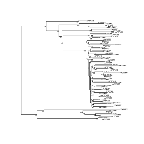
Now we can add the bootstrap supports to the tree.
plotBS(myalignment.tn93.nj,myalignment.tn93.nj.boot$trees,type="phylogram",cex=0.5)

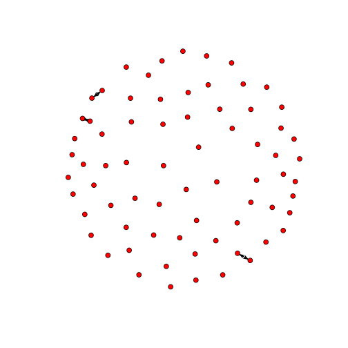
We can also create a network of 'similar' sequences, by defining a threshold distance.
thresh <- 0.01
myalignment.dist.tn93.net <- network(myalignment.dist.tn93<=thresh)
plot(myalignment.dist.tn93.net)
