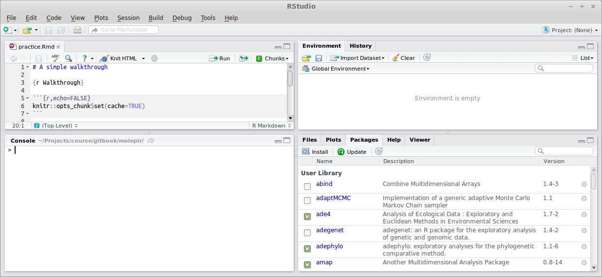
A simple walkthrough

Let's make a tree

In order to help familiarise yourself with R and RStudio, we'll make a tree.

First steps

• Open RStudio.
• Change to the working directory where your files will be kept.
  • Session > Set Working Directory > Choose Directory

Installing libraries

We will use several libraries in this course, most of which have already been installed for you. However, it's good to know how to install them yourself.

• Use the install.packages command.
• Use Packages tab in the lower left hand panel.

Loading libraries

Most libraries are not loaded by default, so you'll need to load them yourself. Try the following command

library(ape)

Sequence data

Most of the time, we will use FASTA formatted sequence data.

>SequenceName
CTCTTGGCTCTGTTGTCCTGTTTGACCATCCCAGCTTCCGCTTATGAAG
CATGTCACAAACGACTGCTCCAACTCGAGCATTGTCTATGAGGCAGCGG
TGCGTGCCCTGTGTTCGGGAGGGCAACACCTCCCGCTGCTGGGTATCGC
AACTCCAGTGTCCCCACCACGACGATACGGCGCCATGTCGATTTGCTCG
GCCATGTACGTGGGGGATCTCTGCGGATCTGTTTTCCTCGTCTCCCAAC
TATCAGACGGTACAGGACTGCAATTGTTCAATCTATCCTGGCCACGTAA

Reading in sequence data

• A dataset we will use throughout is of partial hepatitis C sequences of the Core/E1 region, sampled from Egypt (Ray, Arthur, Carella, Bukh, and Thomas, 2000).

myseqs <- read.dna("ray2000.fas",format="fasta",as.matrix=TRUE)

• R uses <- to assign to names
• The function in R to read in DNA sequences is read.dna
• We can learn more about this function by typing ?read.dna
• If we can't remember the name, we could search for matches e.g. ??dna
• The help tells us that we have to specify the format, as well as whether to read the data into a matrix
• These sequences are aligned, so we set use.matrix=TRUE

What happened?

Nothing happened! This is because nothing went wrong. If we want to see the data, we can just type in the name we gave it.

myseqs

## 71 DNA sequences in binary format stored in a matrix.
## 
## All sequences of same length: 411 
## 
## Labels: AF271819 AF271820 AF271821 AF271823 AF271824 AF271822 ...
## 
## Base composition:
##     a     c     g     t 
## 0.177 0.305 0.256 0.262

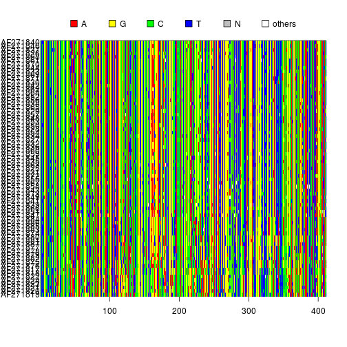
Displaying the alignment

image(myseqs)

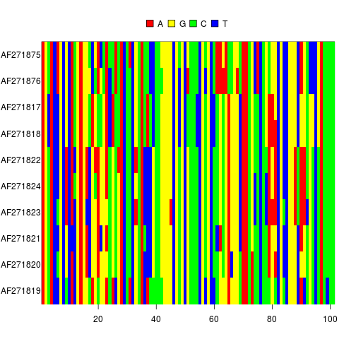
Displaying part of an alignment

image(myseqs[1:10,100:200])

Generating a distance matrix

• Several algorithmic approaches for obtaining genetic distances
• The command below generates a distance matrix using the Tamura-Nei (1993) distance

myseqs.dist <- dist.dna(myseqs,model="TN93")

Reconstructing a neighbour joining tree

• The nj command generates a neighbour joining tree from a distance matrix.

myseqs.njtree <- nj(myseqs.dist)
myseqs.njtree

## 
## Phylogenetic tree with 71 tips and 69 internal nodes.
## 
## Tip labels:
##     AF271819, AF271820, AF271821, AF271823, AF271824, AF271822, ...
## 
## Unrooted; includes branch lengths.

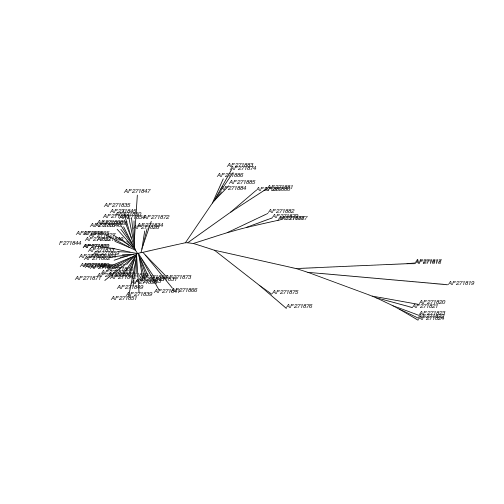
Plotting a tree

plot(myseqs.njtree,type="unrooted",cex=0.5)

Questions and concerns: implementation

• 'I can't remember all that typing'...
• 'I can make a tree more easily using a graphical interface, such as in MEGA'...

Literate programming

• R and RStudio have good support for literate programming
  • Mixture of text and code
• Rather than type everything from scratch, we place all commands in a text file