- Introduction
- 1. Background
- 2. Retrieving sequences
- 3. Sequence alignment
- 4. Distance-based analyses
- 5. Recombination
- 6. Maximum likelihood based analyses
- 7. Visualising trees
- 8. Time-stamped phylogenies
- 9. Bayesian reconstruction of time trees
- 10. Effective population size estimation
- 11. Structured populations
- 12. References
- Published with GitBook
'Mugration' exercise
Load the libraries.
library(ape)
library(phangorn)
library(ggtree)
##
## Attaching package: 'ggtree'
##
## The following objects are masked from 'package:IRanges':
##
##     collapse, expand
##
## The following object is masked from 'package:phangorn':
##
##     getRoot
Load the FASTA data.
myseqs <- read.dna("H5N1.fas",format="fasta")
mytree <- nj(dist.dna(myseqs,model="TN93"))
Starting with the neighbour joining tree, we reconstruct a maximum likelihood tree, as we did before. Note that we get a warning about negative branch lengths in the NJ tree, which aren't allowed in the ML tree.
myseqs.phydat <- as.phyDat(myseqs)
myseqs.gtrig <- pml(mytree,myseqs.phydat,model="GTR+I+G",k=4)
## Warning in pml(mytree, myseqs.phydat, model = "GTR+I+G", k = 4): negative
## edges length changed to 0!
myseqs.gtrig <- optim.pml(myseqs.gtrig,optNni=TRUE,optBf=TRUE,optQ=TRUE,optInv=TRUE,optGamma=TRUE,optEdge=TRUE,optRate=FALSE)
## optimize edge weights:  -6050.051 --> -6038.844
## optimize base frequencies:  -6038.844 --> -5986.777
## optimize rate matrix:  -5986.777 --> -5728.631
## optimize invariant sites:  -5728.631 --> -5717.886
## optimize shape parameter:  -5717.886 --> -5717.886
## optimize edge weights:  -5717.886 --> -5717.684
## optimize topology:  -5717.684 --> -5704.969
## optimize topology:  -5704.969 --> -5704.969
## 4
## optimize base frequencies:  -5704.969 --> -5704.725
## optimize rate matrix:  -5704.725 --> -5704.684
## optimize invariant sites:  -5704.684 --> -5704.657
## optimize shape parameter:  -5704.657 --> -5704.657
## optimize edge weights:  -5704.657 --> -5704.657
## optimize topology:  -5704.657 --> -5704.657
## 0
## optimize base frequencies:  -5704.657 --> -5704.655
## optimize rate matrix:  -5704.655 --> -5704.655
## optimize invariant sites:  -5704.655 --> -5704.655
## optimize shape parameter:  -5704.655 --> -5704.655
## optimize edge weights:  -5704.655 --> -5704.655
## optimize base frequencies:  -5704.655 --> -5704.655
## optimize rate matrix:  -5704.655 --> -5704.655
## optimize invariant sites:  -5704.655 --> -5704.655
## optimize shape parameter:  -5704.655 --> -5704.654
## optimize edge weights:  -5704.654 --> -5704.654
## optimize base frequencies:  -5704.654 --> -5704.654
## optimize rate matrix:  -5704.654 --> -5704.654
## optimize invariant sites:  -5704.654 --> -5704.654
## optimize shape parameter:  -5704.654 --> -5704.654
## optimize edge weights:  -5704.654 --> -5704.654
## optimize base frequencies:  -5704.654 --> -5704.654
## optimize rate matrix:  -5704.654 --> -5704.654
## optimize invariant sites:  -5704.654 --> -5704.654
## optimize shape parameter:  -5704.654 --> -5704.653
## optimize edge weights:  -5704.653 --> -5704.653
## optimize base frequencies:  -5704.653 --> -5704.653
## optimize rate matrix:  -5704.653 --> -5704.653
## optimize invariant sites:  -5704.653 --> -5704.653
## optimize shape parameter:  -5704.653 --> -5704.653
## optimize edge weights:  -5704.653 --> -5704.653
## optimize base frequencies:  -5704.653 --> -5704.653
## optimize rate matrix:  -5704.653 --> -5704.653
## optimize invariant sites:  -5704.653 --> -5704.653
## optimize shape parameter:  -5704.653 --> -5704.653
## optimize edge weights:  -5704.653 --> -5704.653
## optimize base frequencies:  -5704.653 --> -5704.653
## optimize rate matrix:  -5704.653 --> -5704.653
## optimize invariant sites:  -5704.653 --> -5704.653
## optimize shape parameter:  -5704.653 --> -5704.652
## optimize edge weights:  -5704.652 --> -5704.652
## optimize base frequencies:  -5704.652 --> -5704.652
## optimize rate matrix:  -5704.652 --> -5704.652
## optimize invariant sites:  -5704.652 --> -5704.652
## optimize shape parameter:  -5704.652 --> -5704.652
## optimize edge weights:  -5704.652 --> -5704.652
myseqs.mltree <- myseqs.gtrig$tree
We need to root the tree in order to do ancestral reconstruction. We could use rtt or lsd, but in principle, we could use any method we discussed before. We scan the names of the tip labels, to get the tip dates and location.
info <- scan(what=list(character(),character(),character(),character(),integer()),sep="_",quote="\"",text=paste(myseqs.mltree$tip.label,collapse="\n"),quiet=TRUE)
tipnames <- myseqs.mltree$tip.label
tipdates <- as.double(info[[5]])
tipdates
##  [1] 2005 2005 2002 2001 2005 2005 2004 2004 2003 2001 2000 1996 2005 2005
## [15] 2004 2004 2004 2004 2004 2004 2004 2004 2004 2001 2001 2004 2003 2002
## [29] 1998 1997 1997 1997 1997 1997 1997 1997 1997 1997 1997 2005 2005 2005
## [43] 2005
We can now root the tree and turn branch lengths into time using LSD.
write.tree(myseqs.mltree,"H5N1.tre")
write.table(rbind(c(length(tipnames),""),cbind(tipnames,tipdates)),"H5N1.td",col.names=FALSE,row.names=FALSE,quote=FALSE)
lsd.cmd <- sprintf("lsd -i %s -d %s -c -n 1 -r -b %s -s %s -v","H5N1.tre","H5N1.td",paste(10),seq.len)
lsd.cmd
## [1] "lsd -i H5N1.tre -d H5N1.td -c -n 1 -r -b 10 -s 6987 -v"
lsd <- system(lsd.cmd,intern=TRUE)
procresult <- function(fn){
  result <- readLines(fn)
  line <- result[grep("Tree 1 rate ",result)]
  line.split <- strsplit(line, " ")[[1]]
  list(rate=as.double(line.split[4]),tmrca=as.double(line.split[6]))
}
procresult("H5N1_result.txt")
## $rate
## [1] 0.003233
##
## $tmrca
## [1] 1994.113
lsd.tree <- read.tree("H5N1_result_newick_date.txt")
Now we can extract the location, and reconstruct the changes in state. Here is another R trick to parse sequence headers.
info <- scan(what=list(character(),character(),character(),character(),integer()),sep="_",quote="\"",text=paste(lsd.tree$tip.label,collapse="\n"),quiet=TRUE)
info
## [[1]]
##  [1] "A" "A" "A" "A" "A" "A" "A" "A" "A" "A" "A" "A" "A" "A" "A" "A" "A"
## [18] "A" "A" "A" "A" "A" "A" "A" "A" "A" "A" "A" "A" "A" "A" "A" "A" "A"
## [35] "A" "A" "A" "A" "A" "A" "A" "A" "A"
##
## [[2]]
##  [1] "chicken"   "Goose"     "bird"      "bird"      "bird"
##  [6] "bird"      "bird"      "chicken"   "bird"      "bird"
## [11] "bird"      "duck"      "goose"     "goose"     "goose"
## [16] "duck"      "duck"      "chicken"   "swine"     "chicken"
## [21] "duck"      "goose"     "goose"     "duck"      "chicken"
## [26] "duck"      "Chicken"   "greyheron" "duck"      "duck"
## [31] "duck"      "duck"      "chicken"   "chicken"   "bird"
## [36] "duck"      "chicken"   "duck"      "duck"      "duck"
## [41] "duck"      "duck"      "Goose"
##
## [[3]]
##  [1] "HongKong"  "HongKong"  "HongKong"  "HongKong"  "HongKong"
##  [6] "HongKong"  "HongKong"  "HongKong"  "HongKong"  "HongKong"
## [11] "HongKong"  "Guangxi"   "Guangxi"   "Guangxi"   "Guangxi"
## [16] "Guangxi"   "Guangxi"   "Guangxi"   "Fujian"    "Fujian"
## [21] "Fujian"    "Guangdong" "Guangxi"   "Hunan"     "Guangxi"
## [26] "Guangxi"   "Guangdong" "HongKong"  "Guangxi"   "Hunan"
## [31] "Hunan"     "Hunan"     "Guangdong" "Guangdong" "HongKong"
## [36] "Guangxi"   "HongKong"  "Guangdong" "Guangdong" "Guangxi"
## [41] "Fujian"    "Guangdong" "Guangdong"
##
## [[4]]
##  [1] "915"  "w355" "488"  "97"   "481"  "485"  "514"  "258"  "503"  "542"
## [11] "532"  "1378" "914"  "1097" "2112" "2291" "1681" "2439" "F1"   "1042"
## [21] "897"  "2216" "345"  "1265" "2461" "793"  "810"  "837"  "351"  "139"
## [31] "182"  "157"  "191"  "174"  "213"  "50"   "863"  "4610" "01"   "22"
## [41] "13"   "12"   "1"
##
## [[5]]
##  [1] 1997 1997 1997 1998 1997 1997 1997 1997 1997 1997 1997 2004 2004 2004
## [15] 2004 2004 2004 2004 2001 2005 2005 2005 2005 2005 2004 2005 2005 2004
## [29] 2004 2005 2005 2005 2004 2004 2003 2001 2002 2003 2001 2001 2002 2000
## [43] 1996
The location is the third entry in the list.
mylocation <- as.factor(info[[3]])
mylocation
##  [1] HongKong  HongKong  HongKong  HongKong  HongKong  HongKong  HongKong
##  [8] HongKong  HongKong  HongKong  HongKong  Guangxi   Guangxi   Guangxi
## [15] Guangxi   Guangxi   Guangxi   Guangxi   Fujian    Fujian    Fujian
## [22] Guangdong Guangxi   Hunan     Guangxi   Guangxi   Guangdong HongKong
## [29] Guangxi   Hunan     Hunan     Hunan     Guangdong Guangdong HongKong
## [36] Guangxi   HongKong  Guangdong Guangdong Guangxi   Fujian    Guangdong
## [43] Guangdong
## Levels: Fujian Guangdong Guangxi HongKong Hunan
We fix any small branch lengths.
lsd.tree$edge.length[lsd.tree$edge.length<0.00000001] <- 0.00000001
Now perform ancestral reconstruction of the location; I use a simple equal rates model (model="ER"), although in principle I could use more complex ones.
lsd.tree.ace <- ace(mylocation,lsd.tree,type="discrete",method="ML",model="ER")
lsd.tree.ace
##
##     Ancestral Character Estimation
##
## Call: ace(x = mylocation, phy = lsd.tree, type = "discrete", method = "ML",
##     model = "ER")
##
##     Log-likelihood: -45.57865
##
## Rate index matrix:
##           Fujian Guangdong Guangxi HongKong Hunan
## Fujian         .         1       1        1     1
## Guangdong      1         .       1        1     1
## Guangxi        1         1       .        1     1
## HongKong       1         1       1        .     1
## Hunan          1         1       1        1     .
##
## Parameter estimates:
##  rate index estimate std-err
##           1   0.0701  0.0151
##
## Scaled likelihoods at the root (type '...$lik.anc' to get them for all nodes):
##     Fujian  Guangdong    Guangxi   HongKong      Hunan
## 0.02836587 0.20304071 0.02992778 0.71128212 0.02738351
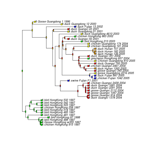
plot(lsd.tree, type="p",label.offset=0.0025,cex=0.75)
co <- c("blue", "yellow","red","green","orange")
tiplabels(pch = 22, bg = co[as.numeric(mylocation)], cex = 1.0)
nodelabels(thermo = lsd.tree.ace$lik.anc, piecol = co, cex = 0.25)
The next steps in this analysis could be:
- To explore different possible models for the migration process
- To perform a joint trait/tree analysis in BEAST (see here for an analysis of the same data)
- To develop more complex structured coalescent models e.g. in
rcolgem